"AN INVESTMENT IN KNOWLEDGE ALWAYS PAYS THE BEST INTEREST" BENJAMIN FRANKLIN
"AN INVESTMENT IN KNOWLEDGE ALWAYS PAYS THE BEST INTEREST" BENJAMIN FRANKLIN

Research Article - (2022) Volume 59, Issue 2
Received: Jun 13, 2022, Manuscript No. BSSJAR-22-66536; Editor assigned: Jun 15, 2022, Pre QC No. BSSJAR-22-66536; Reviewed: Jun 29, 2022, QC No. BSSJAR-22-66536; Revised: Jul 06, 2022, Manuscript No. BSSJAR-22-66536; Published: Jul 16, 2022, DOI: 10.36962/GBSSJAR/59.2.009
Electrocardiography (ECG) is a commonly used diagnostic method that is based on reading electrical potentials from the prescribed epicardial potentials is a well-posed forward problem and involves solving Laplaces's equation in the source-free volume between the torso and heart surface. Computation of epicardial potentials from torso potentials is the corresponding inverse problem. In our study, the two-dimensional model is manipulated to create epicardial model with inhomogeneous version. The model is separately meshed using the mesh generator tool of COMSOL package. The resulting mesh data are transferred to our Python code. In our mesh, the torso potentials are measured at 29 nodes that correspond to the locations of pericardial leads in standard ECG and in epicardial simulations, the epicardial potentials are measured at 24 nodes. Reconstruction of the epicardial potentials have been accomplished successfully with 4 different types of regularization methods named TSVD, zero order, first order and mean value Tikhonov regularizations.
betsat bettilt vegabet betkanyon matbet celtabet hilbet melbet kingbetting wipbet pusulabet superbahis lidyabet holiganbet 1xbet asyabahis jetbahis betdoksan betetebet betgram
Electrocardiography, Epicardial potentials, Forward problem, Inverse problem, Regularization methods.
The electrical activity of the heart can be modeled using mathematical approaches at different levels. At cellular level, membrane potential models are proposed for different cell types in the heart. The predictive power of such methods has provided the researchers with a vast knowledge about the functioning mechanism of the heart (Buist M and Pullan A, 2002). Many health problems associated with the heart are related to the disturbances occurring in the electrical activity of the heart. As a result, different heart problems can be diagnosed with electrocardiogram, or ECG, which is a relatively simple noninva (Shahidi A V, Savard, P and Nadeau R, 1994). In many studies, the heart is removed from problem domain; instead, potential boundary conditions applied to the outer surface of the heart surface (epicardial potentials) that would impose the effect of the heart to the problem. The epicardial potentials can be measured during open chest surgery on a patient or in experiments with animal hearts places in electrolytic tanks (Tuboly G, Kozmann G, Maros, I 2015). Calculation of the torso potentials from the prescribed epicardial potentials is a well-posed forward problem and involves solving Laplaces's equation in the source-free volume between the torso and heart surface. Computation of epicardial potentials from torso potentials is the corresponding inverse problem (Pullan A 2005, Lines G 2003 and Bradley, C 2000). A major objective of contemporary research on this inverse ECG problem is clinically-relevant simulations using torso and heart models that are realistic and subject-specific in biophysical and anatomical aspects
Forward problem of electrocardiography
Forward problem of ECG can be formulated in the simpler case; heart is removed from the problem domain leaving a pericardial inner surface. The effect of the heart is introduced to the problem by imposing realistic pericardial potentials to this surface as a boundary condition. This amounts to a Laplace PDE to be solved in the torso domain.
Human body is a volume conductor, where capacitive and inductive effects are relatively weak. Considering the frequencies at which the heart operates, time-dependence may be ignored. In other words, at each time instant, the electrical activity of the heart can be regarded as static, a case often named as quasi-static (Shahidi A V 1994, Gulrajani RM 1998 and Pullan, A 1996).
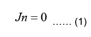
Since the body is surrounded by non-conducting air, the normal component of the current must be zero at the body surface, meaning:
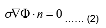
Where n is the outward unit normal of the body surface. According to case of quasi-static fields, the boundary condition can be written as:
The electrostatic problem can now be stated as:
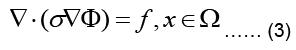
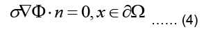
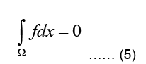
Where Ω represent the problem domain, which is the entire body including the heart in our case, and ∂Ω is the boundary of the problem domain, i.e. the body surface. f is the source term indicating charge creation. Since no net charge is created in the body:
It should be noted that the conductivity σ is generally inhomogeneous throughout the body, since different types of tissues have different chemical composition and conductivities (Shahidi A V 1994 and Gulrajani RM 1998).
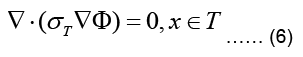
The torso, denoted as T, is a passive conductor since it does not contain any current sources, meaning:
where σT refer now to torso conductivity and potential, respectively. The torso is surrounded by nonconducting air such that the normal component of the current density vector on its outer
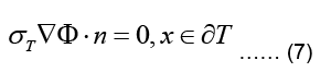
This type of boundary condition involving the gradient of the main variable is called a Neuman boundary condition.
The inner boundary of the torso, denoted as ∂H, interfaces the heart (Geneser SE, 2006). Due to the continuity of the potential across boundaries of different media, we assume that the potential distribution on the inner torso boundary matches with the pericardial potentials which gives:
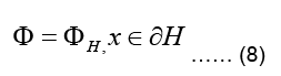
Where ∂H is the pericardial potential distribution on the outer heart surface (Buist M and Pullan A 2002, Shahidi A V 1994, Gulrajani RM 1998 and Geneser SE 2007). The boundary condition in Eq.(8), where the value (and not value of its gradient) of the main variable is set, is called a Dirichlet boundary condition (Buist ML and Pullan A J, 2003).
Finite element formulation of the torso problem
In the case of the epicardial forward problem, Finite Element Method (FEM) is used to solve the Laplace PDE given in Eq. (6) subject to the boundary conditions given in Eqs. (7,8).
The weighted residual form for this equation is obtained by multiplying Eq. (4) with a weighting function w integrating the resulting term over the problem domain Ω and equating the integral to zero:
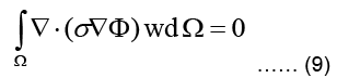
Using the identity, applying Green-Gauss theorem, and also subdividing the domain into L triangular finite elements, Eq. (9) can be written as:
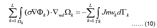
Where Γ represents the boundary of the problem domain. Since a current density J injected to the domain at the boundary fulfills 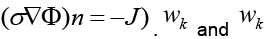 are the solution and the weighting function within the kth element.
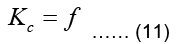
Calculation and assembly of element matrices and vectors will result to Eq. (11):
Note that in the epicardial forward problem, the natural boundary condition is identically zero (meaning f=0) since J=0 (Eq. (7)). The essential boundary conditions represent the epicardial potentials imposed on the epicardial surface.
Geometric model
The two-dimensional geometric model used in this study consists of a single two-dimensional MRI slice image obtained from Utah University. The slice image is taken 50 mm superior to the apex of the heart and processed for the segmentation of lungs, skeletal muscle, fat, and torso cavity (Fig 1). Different conductivity values are assigned to these regions (Table 1).

Figure 1: Two-dimensional geometric model of the torso.
| Organ category | Conductivity value (ms/cm) |
|---|---|
| Lungs | 0.96 |
| Skeletal muscle | 2 |
| Fat | 0.45 |
| Torso cavity | 2.39 |
Table 1. Conductivity values corresponding to organs in the model.
Inverse problem of electrocardiography
To obtain a unique solution and to eliminate the fluctuating nature of the solution, some constraints have to be applied to the solution of the inverse problem. These constraints can cast the solution into a certain functional form, effectively removes certain types of possible solutions and push discussion shows that ill-posed problems, in their original form, are not suitable for performing computer simulations. Application of such constraints that would turn an otherwise irregular solution into a more regular one is called regularization.
We have applied two of these techniques, namely Truncated Singular Value Decomposition (TSVD) regularization and Tikhonov regularization (Shahidi A V Savard P and Nadeau R 1994). There are different variants of Tikhonov regularization that we have employed in the solution of inverse problem, namely 0th order, 1st order and mean value regularization. Mean value regularization, although based on a simple idea, has not been used in inverse ECG problem before.
In actual ECG, torso potentials are measured at a limited number of points. Consequently, the inverse problem is usually formulated in such a way that the epicardial potentials in its entirety are predicted from torso potentials measured at a limited number of points.
To tackle the inverse problem, we first subdivide the nodes of the FE mesh into three groups: a) All nodes on the epicardium, b) torso nodes where surface potentials are measured, c) the rest of the nodes. The values of the corresponding nodal potentials are collected in vectors H, T, and R, respectively. Then, the stiffness matrix K can be reordered and divide into submatrices. It can be rewritten as follows:
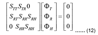
Note that there is no source in the epicardial formulation and thus the global force vector f vanishes. There is no direct connection between the epicardial nodes and torso nodes, and therefore the submatrices STH and SHT are zero in the above expression (Pullan A Buist ML and Cheng L K, 2005). At this point, it is possible to presuppose that the available torso potentials T can be imposed as essential boundary conditions in Eq. (13) and the system can be solved to obtain uHand uR. However, due to the ill-conditioned nature of the problem, this would result to unrealistic, fluctuating potentials in uH
Instead, Eq. (13) is manipulated to directly relate the input to the output, i.e. uT to uH, to give:
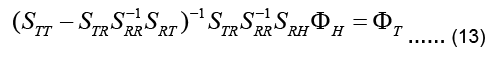
The coefficient matrix on the left-hand side is called the transfer matrix KT:
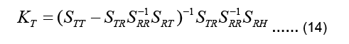
Equation 13 can be now written as:
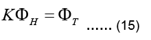
The linear system above is not a square system in general. If torso potentials are available at m nodes and the epicardial potentials are sought for at n nodes, then KT is an m Ë? n matrix,, i.e. 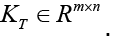 Since n≠m in practice, the system described by Eq. (15) is either an underdetermined system or an over determined system with differing number of unknowns and equations. Furthermore, KT is an ill-conditioned matrix. It is not possible to find a viable solution to Eq. (15) without applying some constraints, i.e. without regularization.
In the forward analysis examples, the epicardial potential distribution shown in Fig 2. Has produced a torso potential distribution for inhomogeneous torso model (Fig 3). For the inverse analysis, now the torso potential is taken as input to estimate the epicardial potential given in Fig 2. Reconstruction of the epicardial potentials have been accomplished successfully with TSVD, and zero order, first order and mean value Tikhonov regularizations. A comparison of these four approaches (Fig 4) indicates that there is no appreciable difference between their performances.


Figure 2: Potentials enforced at 24 epicardial nodes in the forward problem simulations.

Figure 3: Potentials (mV) in homogeneous torso model. The mesh has 4299 nodes and 8154 elements.

Figure 4: Comparison of different approaches in the reconstruction of the epicardial potentials. Note:  Experimental Epicardial Potential;
 Order Tikhonov Reg
The final goal of the ECG inverse problem will be to recover the details of the activation and repolarization process of the myocardium and conduction system. From a clinical point of view, it will be desirable to characterize the heart sources in higher accuracy with fewer body surface leads. In recent years, this approach has advanced to the level of human clinical studies, such as understanding heart activation and repolarization; diagnosing ventricular tachycardia, and arrhythmia; and planning cardiac resynchronization therapy.
[Crossref] [Google Scholar] [Pubmed]
[Crossref] [Google Scholar] [Pubmed]
[Crossref] [Google Scholar] [Pubmed]
[Crossref] [Google Scholar] [Pubmed]
[Crossref] [Google Scholar] [Pubmed]
[Crossref] [Google Scholar] [Pubmed]
[Crossref] [Google Scholar] [Pubmed]